📊 Tests to see if the data meet a normal distribution
Parametric hypothesis tests have as a condition compliance with normality and for this it will be necessary to test this assumption. There are several tests to check the normal distribution, some more powerful than others and in this article we will name the main and best tests when it comes to checking normality. Through a simulation process, the power of each of the tests can be estimated using samples that come from known distributions, but yes, we can measure in each of these samples how far they are from normality.

Experience leads us to think that a moderate deviation from normality is not exactly of great importance in the tests of parametric hypotheses and that they can be carried out without major problems. But there are circumstances in which it is not possible to avoid such non-compliance and for these cases, there are two types of alternatives. The first is to use non-parametric statistics and the second is to use equivalent methods, in these cases no assumptions are required regarding the distribution of the data. But if the assumption of normality is fulfilled even in an approximate way, the use of parametric methods is much more recommended, since they are much more powerful than non-parametric methods.
Many times some mathematical function is used that is capable of transforming the data in such a way that the new values can fulfill the required assumption. After the data is transformed, the new values are checked again to see if they meet the normality assumption.
The Shapiro Wilk test for many is one of the best options, since its power is very high, with the exception that it is used only for those non-normal distributions that are large enough and with strong distances. For small sample distributions and weak deviations, almost none of the usual tests appear to be good enough. Tests based on equivalence approaches can also be used and most likely, they may be somewhat better than the tests mentioned above.
Most of the techniques used in statistical inference such as hypothesis testing, regression analysis, forecasting models, etc. They are based on parametric models and, as we know, these models are subject to the assumption of normality. We can find in the literature several hypothesis tests proposed in order to verify whether or not the data come from a normal distribution, there are approximately 40 tests developed for this purpose and in the face of this wide range of options, the rigorous question with which we finds the researcher, is which of these tests is the best alternative to check the assumption of normal distribution in his data.
Multiple investigations have been developed in order to establish some criteria for comparison, which allows the researcher to objectively determine which is the most appropriate test. The comparison criterion most used by researchers is based on estimating through a simulation process the power that the different normality tests have, in order to recognize those tests whose power is the highest for their investigation. To estimate the power of 33 tests with different sample sizes such as n = 25, 50, 100 whose significance levels are α = 0.05 and 0.1, different symmetric non-normal distributions were used such as: Cauchy, Beta, Laplace, Student’s t, Logistics and also other asymmetric ones such as Gamma, Chi square, Weibull, Log Normal, and Gumbelt) and others with modified normality such as mixed normal, contaminated normal, truncated normal and normal with atypicals to ensure the condition of non-normality . The power in all these cases does not change too much, regardless of whether they have different levels of significance. However, no specific test could be determined as the most powerful, as there are many different options based on the non-normal environment.
Another study that was even more detailed than the one previously mentioned, Shapiro Wilk together with Jarque Bera, was also carried out, in which the same distributions that simulated non-normal samples were used and were determined for the case of symmetric samples, being the most powerful tests. For these symmetric samples, Shapiro Wilk and Anderson Darling were used, which in this case were the best option.
In another investigation, sample sizes with n = 20, 30, 40, 50 were used and it was possible to determine that the samples generated from a Beta distribution, the most powerful test ultimately turned out to be that of Anderson Darling and in the case of samples generated by a Log Normal or a Gamma, the most powerful test ended up being that of Jarque Bera.
In all these studies, in order to estimate power, samples were sought such as the probability distribution that, being not normal, most of them tend to normal in some way and that is why they can affect the results found. On the other hand, in a real analysis, the available data should not necessarily conform to some previously known non-normal distribution, such as those we present in previous studies, since in some cases its distribution will be totally unknown.
Although it is true that generating unknown samples is as important as those samples that come from known distributions, however, they have not been presented in the aforementioned investigations. Therefore, the following study is proposed in which, through a stochastic simulation process, the power of 7 normality tests is estimated, using the Fleishman system to generate samples of unknown distribution, but which in turn is known to They are found in the real data and with different levels of contamination and away from normal.
Taking into account previous research and the most common tests of normality established in statistical software, in most of the literature that covers the subject, it is proposed to study the power of the following tests capable of contrasting the following hypotheses:
Ho: The data come from a normal distribution
H1: The data do not come from a normal distribution
Shapiro Wilk test
This test is used to contrast normality in the case that the sample size is less than 50 observations. The idea is to order the sample from smallest to largest and calculate both the mean and the sample variance. If the Shapiro Wilk statistic is less than the critical value obtained in tables, then the null hypothesis is rejected. It is important to take into account that the table is entered with the values of the level of significance and the size of the sample.
In this normality test, it is considered that the normal probability that comes from the adjustment of the sample data for the normal distribution is similar to a linear regression and that is why the diagonal line of the graph fits perfectly, with the difference that this line is similar to the residuals of a regression.
The test statistic to use is:
W = $\frac{b^{2}}{\sum_{i = 1}^{n}{(xi - \overline{x})}^{2}}$
Being the term b = $\sum_{i = 1}^{k}{ai\ \left\lbrack x_{(n - i + 1)} - \ x_{i} \right\rbrack}$ where ai is a coefficient that is tabulated for each sample size, being the position “i” of each observation. On the other hand, the term $\left\lbrack x_{(n - i + 1)} - \ x_{i} \right\rbrack$ is equivalent to the differences obtained when the first from the last value is subtracted, successively from the second from the penultimate value, the third from the penultimate value and so on until the last value is subtracted from the first value. We are going to suppose that we have seven values, then we can conclude that the sequence of differences is going to be the following:
| Observation i | Xi values sorted in ascending order | $$\left\lbrack x_{(n - i + 1)} - \ x_{i} \right\rbrack$$ |
| 1 | X1 | X7 – X1 |
| 2 | X2 | X6 – X2 |
| 3 | X3 | X5 – X3 |
| 4 | X4 | X4 – X4 |
| 5 | X5 | X3 – X5 |
| 6 | X6 | X2 – X6 |
| 7 | X7 | X1 – X7 |
The acceptance zone for the null hypothesis is made up of the values of the test statistic W, which are less than the expected value or the value that is tabulated $W_{(1 - \alpha;\ n)}$
Acceptance zone = W calculated ≤$\ W_{(1 - \alpha;\ n)}$
Let’s go with the first example: Suppose that a factory has an automatic dispenser that is used to fill containers of a medicine whose volume is 16 ml, eight bottles were selected through random sampling and their packaging volume is measured, where the following results are obtained:
16 ml; 15.9 ml; 15.97 ml; 16.04 ml; 16.05 ml; 15.98 ml; 15.96 ml and 16.02 ml
We want to know if the variable of the volume served follows a normal distribution, for this the normality test of Shapiro Wilks is used and the following hypotheses are raised:
Ho = The random variable that represents the volume served does not have a normal distribution
Ha = The random variable represents the volume served has a normal distribution

The steps to follow in the Shapiro Wilks normality test are as follows:
1.- A table made up of the following columns is built:
a. 1st column: All those values that make up the variable studied are listed (i = 1, 2, 3,…, n)
b. 2nd column: The values of the variable are ordered in ascending order (Xi)
c. 3rd column: The values of the variable are ordered in descending order $X_{(n - i + 1)}$
d. 4th column: the values of the 3rd column are subtracted minus those of the 2nd column
e. 5th column: The values of ai that are tabulated are searched for a sample of size n = 8
f. 6th column: It is made up of the product $ai\ \left\lbrack X_{(n - i + 1)} - \ X_{i} \right\rbrack$, that is, the values of the 5th column are multiplied by the 6th column
g. 7th column: ${(Xi - \overline{X})}^{2}$ is calculated
| 1º | 2º | 3º | 4º | 5º | 6º | 7º |
| i | $$X_{i}$$ | $$X_{(n - i + 1)}$$ | $$\left\lbrack X_{(n - i + 1)} - \ X_{i} \right\rbrack$$ | $$ai$$ | $$ai\left\lbrack X_{(n - i + 1)} - \ X_{i} \right\rbrack$$ | $${(Xi - \overline{X})}^{2}$$ |
| 1 | 15,90 | 16,05 | 0,15 | 0,6052 | 0,090780 | 0,0081 |
| 2 | 15,96 | 16,04 | 0,08 | 0,3164 | 0,025312 | 0,0009 |
| 3 | 15,97 | 16,02 | 0,05 | 0,1743 | 0,008715 | 0,0004 |
| 4 | 15,98 | 16,00 | 0,02 | 0,0561 | 0,001122 | 0,0001 |
| 5 | 16,00 | 15,98 | -0,02 | 0 | 0 | 0,0001 |
| 6 | 16,02 | 15,97 | -0,05 | 0 | 0 | 0,0009 |
| 7 | 16,04 | 15,96 | -0,08 | 0 | 0 | 0,0025 |
| 8 | 16,05 | 15,90 | -0,015 | 0 | 0 | 0,0036 |
| $\sum total$ | 0.0159 | 0,0166 |
The test statistic is obtained by dividing the square of the sum of the values in the 5th column $b^{2}\ $= $\left( \sum_{i = 1}^{k}{ai\ \left\lbrack x_{(n - i + 1)} - \ x_{i} \right\rbrack} \right)^{2}\ $ between the sum of the 6th column $\sum_{i = 1}^{n}{(Xi - \overline{X})}^{2}$
W = $\frac{b^{2}}{\sum_{i = 1}^{n}{(Xi - \overline{X})}^{2}}$ = $\frac{{(0,0159)}^{2}}{0,0166}$ = 0,9553
The acceptance zone for the null hypothesis is obtained by contrasting the value of W (0.95; 8) with the critical value obtained in the tables. To obtain the value in the tables, it must be entered with the level of significance and the number of observations:
As we can see with a significance level of α = 0.05 and n = 8, we obtain a critical value of 0.818. The decision rule to know if we are within the acceptance zone is to compare both values and if the Wcal ≥ Wcritical, the null hypothesis must be rejected. In this case, it is indeed what happens, since:
0.9553 ≥ 0.818
So we can conclude that the null hypothesis is rejected with a confidence level of 95% and therefore, the alternative hypothesis is accepted. This implies that the variable representing the volume served is normally distributed.
We now go with a brief introduction to the Kolmogorov Smirnov normality test. It cannot be compared to the Shapiro Wilks test, since for Kolmogorov Smirnov both the mean and the variance must be known and it cannot be estimated solely from the data, on the other hand the Shapiro Wilks test can be used in samples whose mean and variance are not specified.
The Kolmogorov Smirnov test makes it possible to compare whether the sample score follows a normal distribution or not. This test is part of a group of so-called goodness-of-fit tests, the main characteristics of which are that they pose a hypothesis regarding fit or independence, the mean of the variables is low (ordinal), they do not have excessive restrictions, they are robust and applicable to small samples.
The Kolmogorov Smirnov test is a test that belongs to statistics and that aims to extract information regarding populations. It is used to corroborate whether the scores obtained from a sample follow a normal distribution. Thus, it allows to measure the level of agreement that exists between the theoretical distribution and the distribution of the data set. The objective of this test is to indicate if the data come from a population whose theoretical distribution is specified, therefore, it reasonably tests whether the observations could come from this distribution. The rigorous question is: Do the observations come from some sample with a hypothetical distribution?
The idea of the proposal of the null hypothesis and the alternative hypothesis is to demonstrate that the empirical sampling distribution agrees with the population distribution, for this it is established that the hypotheses are:
Ho = establishes that the empirical distribution is similar to the theoretical one
Ha = states that the observed frequency distribution is not similar to the theoretical distribution.
In short, in this case there is no attempt to reject the null hypothesis and it is convenient that it has a good fit and, therefore, that it is similar. On the contrary, the alternative hypothesis as opposed to the null one determines a bad fit and therefore, that the distribution of the data is not similar to the empirical one.
Conditions for using this test: The way to apply the test correctly is by assuming a series of assumptions. The first thing is that the parameters of the distribution have been previously specified and these parameters are estimated from the sample. It is also necessary to assume that the standard deviation and the mean are parameters of a normal distribution. On the other hand, the maximum and minimum values of the sample determine the range of a uniform distribution.
When determining deviations from a hypothetical distribution, the capacity of this test can be greatly diminished. Thus, to achieve its contrast with a normal distribution of estimated parameters, it will be necessary to consider the possibility of complementing the Kolmogorov Smirnov test with the Lilliefors test.
Advantages of Kolmogórov Smirnov
1.- It is more powerful than other goodness-of-fit tests such as Chi square.
2.- It does not require data grouping, so it is easier to use and calculate.
3.- The statistic of this test only depends on the size of the sample, since it is not dependent on the frequency distribution.
Example of the test kolmogorov Smirnov
We are going to apply the steps to follow for this test with a specific example, for subsequent observations simply follow the same steps that are exposed below:
A researcher measured the height of 100 children with an age of five years and wants to know if these observations come from a normal distribution.

The null and alternative hypotheses are established:
Ho = There are minimal differences between the theoretical values and the observed values of the normal distribution
Ha = The values of the theoretical frequencies whose distribution is normal and the observed values are very different.
For probability values that are less than or equal to 0.05, the null hypothesis is rejected and the alternative hypothesis is accepted.
For all probability values greater than 0.05, the alternative hypothesis is rejected and the null hypothesis is accepted.
After the corresponding measurements, the following results were obtained:
| Rank | Length intervals (cm) | f | fa |
| 1 | 90 - 93 | 5 | 5 |
| 2 | 94 - 97 | 21 | 26 |
| 3 | 98 - 101 | 48 | 74 |
| 4 | 102 - 105 | 19 | 93 |
| 5 | 106 - 109 | 7 | 100 |
| Total | 100 |
Where the total average of the sample gives a value of $\overline{X\ }$= 99.2 and its standard deviation is σ = 2.85
The first step is to calculate the expected theoretical values to obtain a normal distribution. For this, it will be necessary to determine the value of Z with the limits of each interval, for example: in the first interval, Z must be calculated for both the lower and upper limits, that is, a Z for 90 and another for 93, but In subsequent intervals, Z should be calculated only for the upper limits, in this case they are: 97, 101, 105 and 109.
To calculate the Z values, you need to use the following formula:
$Z_{90}$= $\frac{X1 - \ \overline{X}}{\sigma}$ = $\frac{90 - 99,2}{2,85}$ = -3,23
$Z_{93}$= $\frac{X2 - \ \overline{X}}{\sigma}$ = $\frac{93 - 99,2}{2,85}$ = -2,18
$Z_{97}$= $\frac{97 - 92,2}{2,85}$ = -0,77
In this way we continue to calculate each of the Z values corresponding to the subsequent upper limits and place them in a table:
Interval limits Z values of interval limits
| Interval limits | Z values of interval limits |
| 90 | -3,23 |
| 93 | -2,18 |
| 97 | -0,77 |
| 101 | 0.63 |
| 105 | 2,04 |
| 109 | 3,44 |
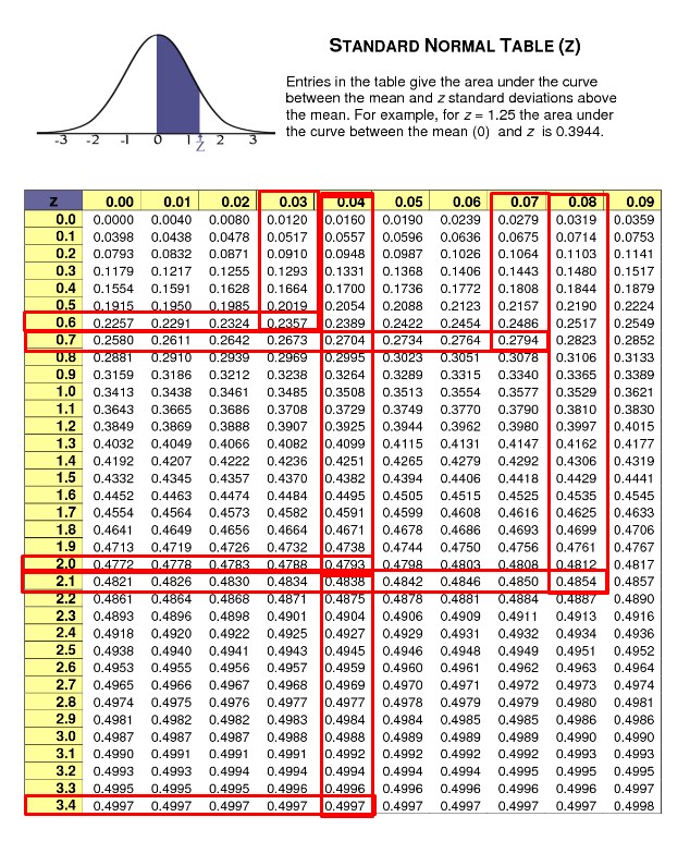
Once all the Z values have been obtained, we must locate the area under the normal curve that is typified in the table. To reach the required value, we must place the whole number with its first decimal place in the left column, and we place the second decimal place in the upper columns and find the value that intersects both numbers. For example, for the first value of Z we have:
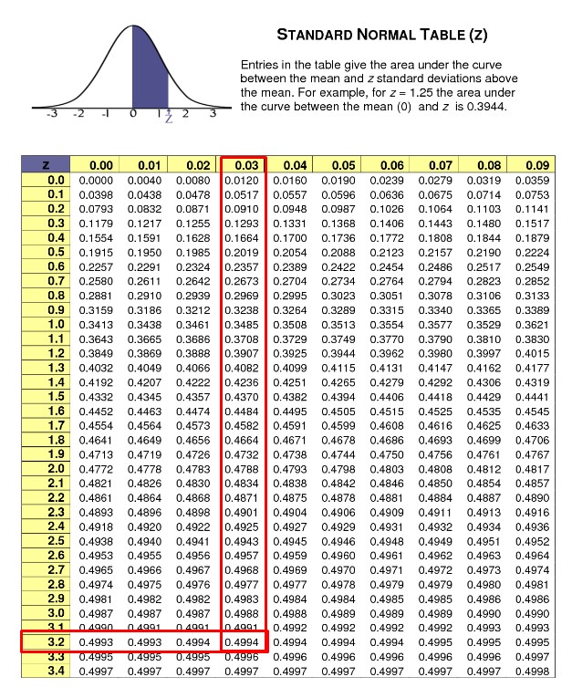
As we can see, we obtain a value of 0.4994 in the table for Z = 3.23, but since it is negative (-3.23) we must also take the value obtained in the table as negative. We carry out the same procedure for the rest of the Z values and obtain the following results that we will place in the third column:
| Interval limits | Z values of interval limits | Typified area under the curve | Differences of areas | Differences x N | fa |
| 90 | -3,23 | -0,4994 | |||
| 93 | -2,18 | -0,4854 | 0,014 | 1,4 | 1,4 |
| 97 | -0,77 | -0,2794 | 0,206 | 20,6 | 22 |
| 101 | 0.63 | 0,2357 | 0,5151 | 51,5 | 73,5 |
| 105 | 2,04 | 0,4793 | 0,2436 | 24,4 | 97,9 |
| 109 | 3,44 | 0,4997 | 0,0200 | 2,0 | 99,9 |
The fourth column is made up of the difference of the standardized values below the area of the curve obtained in the table, for example if we subtract the first two values we have: -0.4854 - (-0.4994) = 0.014. In the same way, the following values are subtracted, with the value of the previous interval, thus filling in the 4th column.
The 5th column is made up of multiplying the differences in areas found in the 4th column by the size of the sample, which in this case is n = 100. For example: 0.014 x 100 = 1.4 we repeat this procedure to the rest of the values, while the 6th column will be made up of the accumulated frequency (fa), that is, the value of the 5th column is added the next value and so on.
In the following table we will show the theoretical frequencies and the observed frequencies that are adapted as follows in the corresponding intervals and then, it is when the Kolmogorov Smirnov method is applied.
Calculation of the D statistic of the Kolmogorov Smirnov test
| Ranks | 1 | 2 | 3 | 4 | 5 |
| theoretical cumulative frequency (ft) | 1,4/100 | 22/100 | 73,5/100 | 97,9/100 | 99,9/100 |
| f cumulative observed (fo) | 5/100 | 26/100 | 74/100 | 93/100 | 100/100 |
| D= ft - fo | -0,036 | -0,004 | -0,005 | 0,049 | -0,001 |
As we can see, the maximum difference in D is 0.049 and this is going to be the value that we are going to compare with the critical value D obtained in the table. The problem is that when we go to the table the maximum value of the number of samples observed in the table is N = 40 in this case N = 100, so we must use the formula for a set of observations greater than 40.
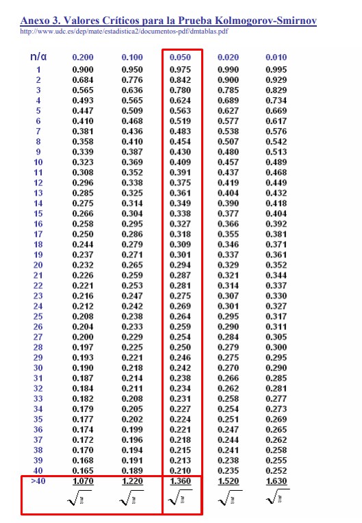
If we use a significance level of α = 0.05, the corresponding formula for the critical value is = $\frac{1,36}{\sqrt{100}}$ = 0,136
Now we must apply the decision rule where the maximum difference of D calculated is compared with the critical value. Given the case of the maximum difference in D calculated is less than the critical value, the null hypothesis is accepted and the alternative hypothesis is rejected. In this case, the maximum difference in D actually calculated is less than the critical value, since:
0.049 < 0.136
Therefore, the null hypothesis is accepted and it can be concluded that there are no significant differences between the calculated theoretical frequencies and the observed frequencies, this implies that the observations have a normal distribution.
Lilliefors test
The Lilliefors test is a correction of the Kolmogorov Smirnov test, which, as we know, is used when the parameters of its hypothetical distribution are known. The problem is that many times it is not so easy to know these values and that is when the Lilliefors test is used with estimates of the mean and standard deviation that are based on the sample data. However, the critical and statistic values will be the same as the Kolmogorov Smirnov test.
Let’s go directly with an example to know how the Lilliefors test is used, suppose we have the following data: 6, 1, -4, 8, -2, 5, 0 and we want to know if they follow a normal distribution considering a significance of α = 0.05 and we can see that the sample size is N = 7
The first step is to order the data from least to greatest: -4, -2, 0, 1, 5, 6, 8
Then we must establish the intervals that exist between these data:
X < -4
-4 ≤ X <-2
-2 ≤ X <0
0 ≤ X <1
1 ≤ X <5
5 ≤ X <6
6 ≤ X <8
8 ≤ X
The third step is to establish the probabilities, for example for the first interval the probability is zero, for the second interval it will be 1/7, for the third it will be 2/7 and thus we are increasing a number in the numerator and dividing it by the number of data, for each of the intervals
0 if X <-4
1/7 if -4 ≤ X <-2
2/7 if -2 ≤ X <0
3/7 if 0 ≤ X <1
4/7 if 1 ≤ X <5
5/7 if 5 ≤ X <6
6/7 if 6 ≤ X <8
7/7 if 8 ≤ X
The fourth step is to calculate the arithmetic mean of the observations in the sample:
$\overline{X}$ = $\frac{- 4 + ( - 2) + 0 + 1 + 5 + 6 + 8}{7}$ = 2
In order to later calculate the standard deviation of the observations and for this, it will be necessary to square the subtraction of each of the observations minus the value of the arithmetic mean and that total is divided by the subtraction of the number of observations minus one (N -1). The square root is extracted from the result of this calculation, the resulting number being the standard deviation:
σ = $\sqrt{\frac{( - 4 - 2)^{2} + {( - 2 - 2)}^{2} + {(0 - 2)}^{2} + {(1 - 2)}^{2} + {(5 - 2)}^{2} + {(6 - 2)}^{2} + {(8 - 2)}^{2}}{(7 - 1)}}$ = 4.43
Now I proceed to calculate each of the Z values with the formula:
Z= $\frac{(X - \overline{X})}{\sigma}$
Z1= $\frac{- 4 - 2}{4,43}$ = -1,35
Z2= $\frac{- 2 - 2}{4,43}$ = -0,9
Z3= $\frac{0 - 2}{4,43}$ = -0,45
Z4= $\frac{1 - 2}{4,43}$ = -0,22
Z5= $\frac{5 - 2}{4,43}$ = 0,67
Z6= $\frac{6 - 2}{4,43}$ = 0,90
Z7= $\frac{8 - 2}{4,43}$ = 1,35
Later I look in the tables of cumulative probability of the standard function in the same way as we did for the previous example, that is, the units of the first decimal in the left column and the second decimal in the columns that are found on top. For example, if Z = -1.35 we will search for -1.3 in the left column and 0.05 between the columns above and the intersection will be the value of interest of the cumulative probability, which in this case will be of: 0.0885. In this way, we are looking for the corresponding values in the table for each value of Z and we can place them in the following table:
| $$X_{i}$$ | $S_{7}$ (X) | $\varphi_{7}$($X_{i}$) | $$ {S_{7}\ \left( X_{i} \right) - \varphi}{7}(X{i})$$ | $$ {S_{7}\ \left( X_{i - 1} \right) - \varphi}{7}(X{i}) $$ |
| -4 | 1/7 = 0,1428 | 0,0885 | 0,0543 | 0 – 0,0885 = 0,0885 |
| -2 | 2/7 = 0,2857 | 0,1841 | 0,1016 | 0,1428 - 0,1841= 0,0413 |
| 0 | 3/7 = 0,4285 | 0,3264 | 0,1021 | 0,2857 - 0,3264 = 0,0407 |
| 1 | 4/7 = 0,5714 | 0,4129 | 0,1585 | 0,4285 - 0,4129 = 0,0156 |
| 5 | 5/7 = 0,7142 | 0,7486 | 0,0344 | 0,5714 - 0,7486 = 0,1772 |
| 6 | 6/7 = 0,8571 | 0,8159 | 0,0412 | 0,7142 - 0,8159 = 0,1017 |
| 8 | 7/7 = 1 | 0,9115 | 0,0885 | 0,8571 - 0,9115 = 0,0544 |
As we can see, the first $X_{i}\ $ is made up of the data ordered from least to greatest.
The second column that we call $\varphi_{7}$($X_{i}$) is made up of the probabilities that we previously established how to calculate them, only that we add the result of the division of the numerator by the denominator.
The third column $\varphi_{7}$($X_{i}$) are the values obtained in the tables for each value of Z, while the fourth column is the calculation of the absolute value of the subtraction of the values obtained in the second column minus the third column $\left| {S_{7}\ \left( X_{i} \right) - \varphi}{7}(X{i}) \right|$.
The last column we obtain the first value always subtracting from zero (0) the first value of the column $\varphi_{7}$($X_{i}$), but the subsequent values are obtained from the absolute value of the subtraction between the value obtained in the previous column of $S_{7}$ (X) minus the value of the next row of the 3rd column $\varphi_{7}$($X_{i}$) and so on.
The next step is to determine the test statistic to be able to contrast the hypothesis and for this the maximum value of the last column must be chosen, which in this case is:
Do = max $\left| {S_{7}\ \left( X_{i - 1} \right) - \varphi}{7}(X{i}) \right|$ = 0.1772
Now we go to the Lilliefors Test Table and we must enter with the values n = 7 for a significance of α = 0.05:
We obtain the value of tables which we will call Dt = 0.3 and it is then that we proceed to contrast the value of the test statistic with that obtained in the table. In case the test statistic (Do) is less than the one obtained in the table (Dt), the null hypothesis is accepted and otherwise, it will be rejected (Ho). We can realize that the test statistic is less than the one obtained in the table, since:
0.1772 <0.3
Therefore, the null hypothesis is accepted and it can be concluded that the data have a standard normal distribution.