🔢 Statistical estimation
Predicting something that is happening or something that has already happened, is ultimately the basis of statistics and is deeply rooted in our daily lives. We can also make estimates around a range of possibilities. When for example we say “I think I can finish this task in about six or seven days”, we are already defining a time interval to complete it.
When it comes to data analysis, we apply certain technical nuances and this article is intended for the specific concept of estimation. We will start with the point estimation, later we will deal with the estimation model, but focusing on intervals.
The point estimate
Estimating in statistics means inferring and it is a process by which we can establish what value a parameter has according to what we can deduce from statistical data. That is, estimating is nothing more than establishing certain conclusions, with respect to the population characteristics and according to the results of the sample.
When we establish a specific value, what we call a point estimate (that is, a point) but with respect to the parameter. In other words, the value that we choose as a parameter is placed on the “X” axis and it is precisely the one that provides us with a specific statistical data and is usually called an estimator. For example, if we use the arithmetic mean of a certain sample, in this case, the arithmetic mean will be the estimating parameter.
It is important not to erroneously conclude that every parameter that is inferred from statistical data ends up being the same function or formula but calculated in the sample. Suppose we want to estimate the population mean, for this we must assign the value of the proportion specifically in the sample, in the same way if we want to estimate the population variance. But we must be very careful since this rule has its exceptions, so it is best not to think that way as a rule or pattern.
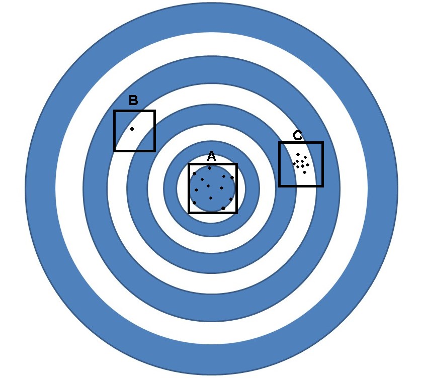
On the other hand, we will call a constant trend bias. Let’s go to an illustrative example, if we affirm that the shotguns found at fairs are specially designed to deviate or miss. We can come to the conclusion that if this deviation is fixed and constant, we can then speak of bias, but if it is not fixed, in this case we will speak of a random variation.
Let’s look at the figure, if the objective is precisely to hit the center of the target, we can speak of a random variation when we refer to the shooting area “A”. But this area cannot be classified as bias thinking of missing, since the shots are precisely around the target.
While in area “B” we can speak of a clear bias, since all the shots are around the same point, but as we can see, that point is not near the center of the target. When we refer to area “C” it is an example of a mixture of both situations, since although it is true that there is a bias, there is also a random variation. This is because the shots are in an area that has some random spread, but all the shots are concentrated around a point that is offset from the center of the target.
In general, the estimators provide a random dispersion, but it is important to take into account that the set that contains all the samples that come from the same population always provide different values. This implies that there is random variation that we have to deal with, as it is unavoidable.
But the situation may be even worse, since it is possible that the chosen estimate has a bias, therefore, not only will it be varying around a point, but also that point around which it varies is not precisely the real population value in the one we are interested in. However, this can be avoided by using estimators that are not biased. For this we will use a resource that is “the expected value”, to achieve this we will use the arithmetic mean, but from our sample distribution of the estimator. The expected value is nothing more than the value (as your phrase implies) that we hope to obtain. It is important then, to choose an estimator so that the expected value specifically matches the parameter. For this, it will be necessary to use the arithmetic mean of the sample, but in this case, we will handle it as an estimator of the population arithmetic mean.
For example, we are interested in knowing how many people will vote for the WW party in the next elections or perhaps, how many cigarettes are consumed in this population for the month of May.

To answer these questions we will use a previous estimate that can come from a proportion or an arithmetic mean. Suppose that the voting population is made up of 1 million inhabitants and we are going to work with a sample of 300 inhabitants, of which 132 of them profess that they will vote for the WW party, this implies that:
We can say that a specific estimate indicates that 44% of the population will vote for the WW party and as there are 1 million inhabitants:
We will then be talking about 440.000 people.
On the other hand, we are going to suppose that an average of 50 cigarettes are smoked per month, taking this as the arithmetic mean of our sample, therefore, the point estimate will indicate that 50 cigarettes will be smoked per person during the month of May. However, we know that there are 1 million inhabitants, so the average will be 50 million cigarettes per month. Therefore, for the estimation of the totals, we do not go down an alternative path, we simply extend the previous estimate of a mean or a proportion.

It is important to emphasize that point estimates when established in the center of the objective are not exactly a good option. Although it is true that they solve certain procedural problems, when the parameter has exactly the legitimized value, it is actually a very difficult coincidence to find.
Let’s go to another specific example, this time we want to know the average time that exists between one breath and another while sleeping. As we all know, we cannot sample all adults over 18 years of age and Europeans, which is the population that interests us, there are too many millions on the continent. So we are going to select a random sample of 350 adults over the age of 18.
After measuring the mean time of our sample, we obtain an average of 5 seconds. If we make a point estimate, we can conclude that the mean time between one breath and another is of course 5 seconds. Suppose for a moment that we can know the precise value that concerns us in that population and that the value is 5.2 seconds, of course we ask ourselves if we have been correct or not, when the difference is 0.2 seconds.
For the majority, they will surely gladly accept either of the two approaches, since the difference is too small to deny the conclusions obtained in the study and in this way, we are not making a point estimate, but thinking about an interval close to 5 which marks an acceptable deviation.
In short, if we fix a point (as we must do for the point estimate) we cannot then use a reasonable interval and continue saying that it is a point estimate, since 5 seconds is not exactly the exact value of the parameter, which as we already know which is 5.2. While it is true that some will not attach importance to them, the estimate is not the true value. That is why point estimates, in the strict sense, tend to err.
In general, what we do in practice are estimates by interval and we use an acceptable range such as “plus or minus”, so the best way to express our result is that a sleeping person takes about 5 seconds between one breath and other. But in statistics that of “more or less” is very imprecise and incomplete, so that we must establish a specific range of what we consider to be our “more or less” to get to be pleased with the result. For example, we can set plus or minus 0.3 seconds and then our conclusion will be an interval of 5 ± 0.3 = {4.7; 5.3} and this is our first example of what an interval estimate is. The set range is what we call “precision error”.
Now, what should we take into account to establish this precision error? When we estimate the mean of a population over an interval, calculating the precision error requires us to have a value, such as the standard deviation of that population. But that is not our objective, we just have no other option to limit it in some way, in order to continue with the process that concerns us.
It is then necessary to make a point estimate, which will consist of establishing a standard deviation of the sample. Suppose you make a bet with a friend that the next person to walk past you is 30 years old. Being your friend, I would accept the bet without hesitation, since if the person passing by is 30 years, 5 months and 2 days old, in the strict sense of the bet, it is not 30 years. So to avoid such inaccuracies, it is always best to use a range.
We are going to establish two different intervals, interval A: a person whose age ranges between 28 and 33 years. An interval B, where the person is between 15 and 50 years old. Of course, if we choose interval B, a person whose age is between 15 and 50 will be much more likely to pass. This denotes that the wider the interval, the more possible results will be integrated and the more likely it is to get it right. This implies that there is a factor within an estimate and that is, security, so the greater the security in an estimate, the more likely I am to be wrong.
Summarizing, we can have three perfectly defined elements in an interval estimation: The initial element, which is of course the estimator, to later establish the precision error that will lead me to be more or less certain.
The sample determines the value of the estimator and it is not something in which we have much interference, but the security, we know, is a function of the choice of our precision error. Therefore, we must choose one of these two remaining options and calculate the value that the other must have. Both elements are related and are inversely proportional, so as security increases, precision decreases and vice versa. Although it is true that achieving this balance is something complex to explain, we can tell you that it also depends on other factors such as habit, tradition and the fear of explaining.
The most logical recommendation in an interval estimation is to start by deciding the security to be reached and depending on it, the precision error value is calculated, to later build the interval.
The advisable process is:
Choosing the ideal safety and precision values, of course, excessively ambitious values will undoubtedly generate very demanding circumstances.
The size of the sample that leads us to achieve these priority objectives of precision and safety must be calculated.
Obtain the sample.
Obtain the statistical value that is going to be used as an estimator and which, therefore, is the one that provides the central point of your interval.
Subsequently, it is calculated in precision error, according to the information provided by the sample and taking into account the desired safety.
The interval is constructed
As we already know, there is no absolute security and the more security we want to obtain, there will always be a price to pay, many times that price will lower the precision or perhaps we will have to take a sample so large that it becomes impossible or very difficult to handle, either because of the cost of time, money, etc.
The best thing then will be to take a fairly reasonable security and it should be closely linked to the consequences of the error that we are willing to assume. For example, if I am depending on the probabilities that a parachute opens or not, the consequences can be fatal, so if my life depends on it, I will demand the maximum possible security.

However, if you sell expensive last generation motorcycles, you may accept the job when the security will be 10%, therefore you will sell one out of every 10 motorcycles. But note that the probabilities in both cases are very different, since the consequences when making a mistake are very different and that is when it will be necessary to place oneself in the specific circumstance when making decisions regarding a value for the safety.

However, this lacks a procedure that manages to limit a specific probabilistic value, they are only general principles. But Ronald Fisher made progress in this regard, it occurred to him that a certain elderly lady was able to differentiate whether the milk or tea had been poured first into a cup of tea with milk, being able to decide just by tasting a small amount of mix.

Fisher decided to limit the amount of successes with which one could come to believe in the lady, of course, we must accept any error on her part. Let’s suppose that we give him 10 cups, the fact that he guesses all of them can happen 1 time out of every 1000 times that we submit anyone to this test, yes, the person in this case is going to get it right by chance and not like the lady, who has some knowledge about it.
Now, if anyone gets it right all but one time, when it comes to determining the order in which the milk tea mixture was composed, it is something that can happen in 1 out of every 100 tests. The fact that two fail will happen 1 out of every 25 times, that is, 4%. That is why Fisher thought of varying the study, where there will be 8 cups, of which half will be served one way and the other half, in the reverse order. It was then that he asked the lady to distinguish them by separating the possibilities into two groups, where he came to the conclusion that when it comes to safety, 95% was a good level. This implies that the lady had a probability with a maximum of 5% of hitting it by chance.
Of that, a little less than 100 years have passed and that value proposed by Fisher, still prevails. In fact, if any researcher decides to use 94%, they should be prepared to answer Why? Since 95% has been assumed as the standard value, but if someone requires greater security, then they resort to 99%, apart from these two values, it is very difficult to find a research work with another security value.
The precision error
The first thing to calculate is the value of the estimator that, as is usually the mean, we will call it (m), the following is ultimately the value of our precision error (ep) and for this we must first establish the security, to which we will call (ø) which will also depend on the particularities of our sample. Once we get to this point, the only thing left is to construct the interval and in this case, it will be necessary to subtract and add to the estimator, our precision value:
There is a parameter to be defined and it is dispersion. One of the examples we mentioned earlier is the number of cigarettes consumed in a town during the month of May. But in this population, everyone smokes the same amount and there is no need to set an interval around a value that does not vary. If all the people smoke exactly 3 cigarettes, then that will be the mean and its variance is zero. So when we have 50 people and each one of them smokes 3 cigarettes per month without exception, the precision value will be zero, this implies that it is not necessary to establish an interval and it is not only a point estimate, but also with a 100% security.
But suppose that we find a population with a completely different situation. In other words, in that population there are many people who smoke an immense amount of cigarettes, while other people smoke absolutely nothing and the rest smoke dissimilar amounts. Now, if we take a sample of 50 people from this new population, we will of course have very different amounts for the number of cigarettes smoked in this population during a month.
This will lead us to the fact that in order to maintain acceptable security, the precision error must be very high, so that the interval is wide enough to include so much variability. In this case, the mean that we have chosen to establish the variation of this characteristic is the standard deviation, but as such characteristic belongs to a variation within the population, then we speak of a standard deviation of the population and we will call it (σ).
So we can say that the precision error will depend on three elements. The first of course is the security level, so the lower the security, the greater the precision error and the larger the interval. The resource to be used to represent safety will be a standardized distance value, which we will call Zsec. But the sample size is missing and we will call it (n), so the larger the sample size, the estimated value will be much closer to the parameter, therefore, the distance between the parameter of the estimated value will be smaller. This is more or less obvious, since the more individuals make up our sample, the more precision we will have when drawing conclusions. Taking into account all the elements, the formula that defines our precision error is:
It is important to take into account that this formula is applied in random samples of very large populations, otherwise, if the population is rather small, the expression of the formula will be different. However, it is very common to use this formula, even with other sampling models.
In statistics this fraction: σ/(√n) It is what is known as the standard error.