♾️ Probabilities
The man usually faces certain situations where he does not have a total control of his certainty and on many occasions we ask ourselves the probability that an event has if it is capable of happening or not, since we do not have absolute certainty that it can happen in some circumstance.
That is why knowing probabilities that can help us measure certainty is so important. Although it is true that statistics is a powerful tool for the knowledge of data, from the way of collecting, presenting and interpreting them in order to generate statistical inferences that help us in making decisions. Probability, on the other hand, is no less important and both are very valuable instruments within the different fields of research, risk markets, productive, administrative and in the health area.
We use the term probability on a daily basis and without the need to become mathematicians. For example, to try to forecast the weather, probability is used, since it deals with both uncertainty and chance. As you will realize later there are three different approaches to probability, but in addition, there are dependent events that tell us to calculate what we call conditional probabilities and what is commonly known as Bayes’ Theorem. But we will also study the development of combinations and permutations.
Many consider that probability is the basis of statistics and even mention that when working with a known population, one can have a better certainty or probability of obtaining a particular sample from that population. That is, the probability is based on a series of rules or patterns where you can have a better idea of what may happen. However, probability has three defined approaches: subjective probability, relative frequency probability and classical probability.
The classical probability is also known as the a priori probability and consists of a sample space where there are results that are mutually exclusive, therefore, it can be said that two or more events cannot occur at the same time, that is, that all situations have the same probability of occurring (equiprobable). When we say that an event A can occur in m ways, we can then say that the probability of A is going to be equal to the number of favorable cases divided by the total number of cases (n).
For example: we are going to suppose that in a box there are 15 white and 8 black marbles. What would be the probability at the time of extracting a marble and that it is black?
Therefore the total number of marbles is n = 23 and that they are black m = 8
The probability that we have to extract a black marble will be 34.78%.

On the other hand, when we talk about relative frequency probability, it is also commonly called a posteriori and as you know it means “after”. This implies that if in a study an event that we call A occurs m number of times, having repeated the event n times, the relative frequency of A would be fr = m / n
When n tends to infinity, since the experiment is repeated several times, the relative frequency will be equal to the probability, in this case A
Let’s go with another example: Let’s suppose that in a racetrack we have observed that horse number 12 has won 9 races out of 10, given the case that you want to bet on this horse of course you want to know the probability that it wins, for this concern:
m = 9 n = 10
Developing:

Answer:
As you will see, the probability that you have of winning when betting on horse number 12 is going to be 90% and what we call subjective probability is determined by the probability that any person assigns to a situation, but based on in your experience.
When any of us forecast the possibility that it rains or does not rain, according to how the sky sees and of course, we are aware that it is not necessarily an absolute pattern, because many times what we predict does not happen, it is a clear example of probability subjective.
From another point of view, it is worth mentioning that many probabilities are calculated axiomatically, understanding that the axioms in probability are those minimum conditions that must be verified, so that a certain function that is defined on a set of events, establishes the consistently your odds.
Now, this relationship that exists between the relative frequency with respect to an event and its probability, through the number of times it is repeated in a large experiment, is attributed to Kolmogorov, who developed the axiomatic theory and relied on 5 theorems and 3 axioms.
Theorems: 1) P (Ø) = 0 2) P (Ā) = 1 - P (A) 3) Being A and B events where A⊂B, then P (A) ≤ P (B) 4) Since A and B are events we can ensure that P(Ā∩B)=P(B)-P(A∩B) 5) Being A and B any two events, P(A∪B) = P(A) + P(B) - P(A∩B)
Axioms:
P(S) = 1
Being A any event, P (A) ≥ 0
Being A AND B events that are mutually exclusive, then A∩B=∅ the probability that either A or B will occur will be P(A∪B) = P(A )+ P(B). Generalizing we can say that if we have several events A1, A2, A3, … An and these events are mutually exclusive, then the intersection of all these events will result in an empty set, while the union will be equal to ∑_(i=1)^n▒P (Ai)
Events
When we make calculations to reach conclusions in some applied science, we generally resort to mathematical models that in turn make up sets of unitary, binary and trinary relations, to satisfy the propositions that are derived from the axioms that are explained with advance.
There are two types of models, the deterministic one in which uncertainty plays no role and the non-deterministic one, which is of the random probabilistic type.
Mathematical calculations are usually applied to solve some type of observable phenomenon of our reality, but also quantifiable and reproducible. Experimentation is the process used to reproduce events and to be able to expect tangible results, with repeatable reproduction being the most important property for this process.
When we talk about deterministic experiments, we can say that they are those in which the conditions of the experiment, manage to allow the results obtained to always be the same. For example, when we put water to heat, we will realize that it always manages to boil or boil at 100 ° C.
While when we talk about non-deterministic experiments, they are those in which the conditions under which the experiment is carried out, are those that determine the probability that the expected results will occur or not, that is, they are those experiments where probability intervenes. For example, when we toss a coin, we cannot predict the expected result with certainty and that is why we must study all the possible results that we will obtain from tossing the coin several times and this is what is called the sample space. The sample space is usually represented by the letter “S” and between braces {} that indicate a set.
Let’s take an example, if we determine the sample space when we flip a coin, as we all know, the coin has two probable sides when it comes to landing. Now, one side of the coin is the head and the other is a tails, for this specific example we will use the nomenclature “C” for heads and “T” for tails, then:
S = {C, T}
But what happens if we flip the coin twice? Our probabilities will be as follows:
S = {CC, CT, TC, TT}

Being “S” the sample space made up of all the possible results of our experiment and can be decomposed into events or events. Both the event and the event are subsets of the sample space and are represented by any letter of the alphabet that is capitalized and with the exception of “S” (to avoid confusion with the symbol of the sample space).
For example, if S = {KKK, KKL, KLK, KLL, LKK, LLL, LKL, LLK} and we intend an “S” event that we will call A in which three K occur, the answer would be A = {KKK} , but if we try an event that we will call B where it is taken into account that it has at least one K, then: B = {KKK, KKL, KLK, KLL, LKK, LKL, LLK}.
In many cases the simplest thing is to try to represent the sample space through Venn diagrams, since in this way those events that can generate other events can be better appreciated.
Venn diagrams are the schematic representation of set theory and are used in logic, mathematics, and diagrammatic reasoning. In Venn diagrams, sets of elements are shown by closed lines.
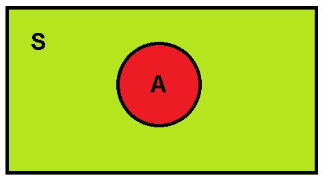
These diagrams were devised by John Venn around 1880 and they try to represent what the sample space “S” is and how we can observe, this space is the one that is part of the rectangle but is not part of the circle, that is, the Venn diagram represents all the points that make up the sample space, but are not included in A.
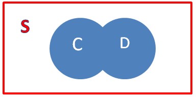
Now, when we join two events such as C and D, we can define the union of the two events, as the set that includes all the points that are in both events and is represented mathematically with the symbol U, therefore it would be C∪D and looks like this:
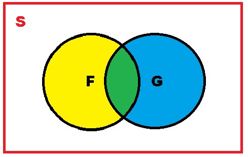
Now, the intersection that exists between two events F and G is represented by those points in the sample that are common to both events and are represented in the following figure by the green area and are mathematically represented as follows F∩G, by both the area that is shaded in green will be:
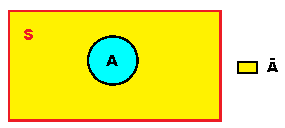
The complement of A, are those points that belong to S but are not in A and is represented by the symbol Ā.
Let’s go with an illustrative example, the sample space for the toss of a die is S= {1, 2, 3, 4, 5, 6}, If we determine three events such that A = {1, 3, 5], in addition B = {4, 5} and C = {1}, we can conclude that:
The complement of A will be: Ā = {2, 4, 6}.
If we require A U B, we need to join all the points of both A and B: A U B = {1, 3, 4, 5}
If what we need is to find, we must find the common points of both events and therefore: A∩C = {1}
Conditional probability
Before understanding what conditional probability is, we must know that there are independent events and dependent events. When a certain event does not exert any type of effect with respect to the probability that another event occurs, it is what we define as an independent event. For example, when it comes to rolling a die, the result that we obtain when we make the first roll, we know that it does not affect in any way the probability that is obtained from a second roll.
Being the events A and B independent, we can express them as follows:
On the other hand, dependent events indicate that one event happens or does not happen with respect to another and it is precisely in this type of event that we use conditional probability, which is the one where situations that are similar and in which it is required to find the probability of event A, but yes, when we already know what happened in another event B.
Now, since A and B are two specific events within a sample space and the condition that P(B) > 0 is obtained, this implies that the probability of A with respect to B is:
An example can clarify the above much more, if we want to calculate the probability when tossing a coin 2 times and also that the result of the second toss when falling to the ground turns out to be heads, when the result of the first toss is a tails. . We must first specify the nomenclature to use and we will use the same that we established in the example mentioned before: C = Heads T = Tails
In this case the sample space is: S = {CC, CT, TC, TT}
To know the conditional probability, we must express the following: P (C Ι T) = P (C ∩ T) / P (T)
It is important to take into account only the sample space in those results where the first toss is a stamp or a cross (T) T = {TC, TT}
When we express the event C ∩ T we will need to limit the sample space, but this time when the second toss has yielded as a result. C = {CC, TC}
When it comes to intersecting C with T, we have one element in common: C ∩ T = {TC}
As we can see, in the original formula there is a division that is carried out precisely with the results that we have just obtained and also we only have 1/4 in the numerator, since we have one element of the 4 that are part of the sample space (in this case TC) of the intersection that exists between T and C. On the other hand, we obtain two elements such as TC and TT from the limited sample space of T, therefore that account gives us 2/4, since they are two elements of the 4 that make up the sample space, therefore:
Answer: according to the calculations when we toss a coin twice, the probability that we will get heads on the second toss is 50%, yes, when we get tails or tails on the first toss.
What probabilities do we have when two events intersect?
When we have an event A and another B, given the case that the intersection between the two generates a new event, where all the points of the sample are common to both A and B. It is important to take into account that when we talk about the intersection of both events, we refer to the event composed of those common elements of two or more events when they intersect and therefore, the probability will only be equal to the probability that the common elements have. According to the property that the intersection of sets has, we can say that: A ∩ S = A A ∩ ∅ = ∅ A ∩ Ā = ∅ With B ⊂ A we can then say A ∩ B = B
Let’s now go with an example, suppose that a dice is thrown into the air and we want to analyze two events, the first event is that an odd number is returned and the second is that the number is less than 4 Let’s first define the nomenclature: I = odd number A = less than 4 We then have that: I = {1, 3, 5} A = {1, 2, 3}
Answer: As we already know, this problem takes us directly to an intersection of probabilities, we must then find the elements in common of I and A, if we observe we can realize that they are the numbers 1 and 3, this implies that we obtain 2 of the 6 points that make up our sample space, therefore: P (I ∩ A) = 2/6 P (I ∩ A) = 0.3333
Answer: The probability that we have when we throw a dice into the air and that a number that is odd will fall and is also less than 4 is 33.33%.

Bayes theorem
As we saw in a previous article, Bayes’ theorem allows us to calculate the probability of an event A, but from what happens in an event B. This theorem is generally used in areas such as quality control In this way, we can know how likely we are to find a defective item or, on the contrary, that it is perfectly manufactured.
According to Bayes’ formula, we can assume that we have a sample space “S” which in turn is made up of “n” events, but in addition, each of the events are mutually exclusive. Of course, the union of all the events will make up our sample space “S”.
On the other hand, we can suppose that H is any event that is in “S”, where P(H) > 0, so that the conditional probability that H generates on other events such as: G1, G2, G3, …, Gn can be expressed through the Bayes formula:
In order to better visualize the Bayes formula. It is advisable to rely on what we call a probability tree, which is nothing more than a graphical representation where we can visualize the groupings of the elements that influence the formula.
For example: A small company dedicated to the manufacture of clothing, depends in turn on other companies that send the prefabricated pieces, in this sense, the small company has three suppliers that are: Mr. Oliver who provides 60% of the clothing, while Mr. Jack supplies 30% and the rest is produced by Mr. John.
According to his experience, the president of the company assumes that the probability of obtaining a defective pants from Mr. Oliver is 4%, in the same way, he believes that the probability corresponding to Mr. Jack is 9% and the John’s is 7%. All suppliers deliver their ready-made garments the same day and at that moment they find defective pants from which supplier is the defective pants most likely to come from?
First, a probability tree is made so that the probability paths can be illustrated:
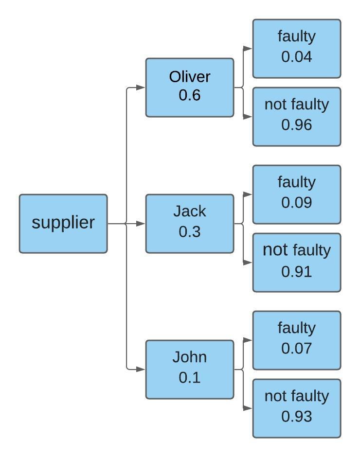
Once the probability tree has been visualized, the path of each provider is followed, in this case the name of each of the providers and then multiplied by the data of interest, for this specific case it will be the defective path of that supplier and finally, that result is divided between all the branches of the defective cases, that is, the sum of all the suppliers.
Let’s suppose that we want to know the probability that the defective pants were manufactured by Mr. Oliver:
According to the formulas we can conclude that Mr. Oliver has a 41.37% probability at the time of having manufactured the defective pants.
Now, if we want to know the probability that the defective pants come from Mr. Jack, we must carry out the same procedure:
As we can see, Mr. Jack has a 46.55% probability of having made the defective pants. Finally, we need to know the probability that Mr. John has of having manufactured the defective part.
This calculation indicates that Mr. John has a 12.06% probability of having made the defective pants.
Answer: As we can see, it is most likely that the defective pants come from the manufacturer named Jack, since this supplier has a probability of 46.55% and therefore, this number is higher than that of the other two manufacturers.
Counting techniques
When we calculate a probability, it can become tedious or complicated to count the elements that make up the set, that is why it is advisable to apply techniques that favor us when carrying out a count and also that allow us to solve and know some problems in as far as probabilities are concerned.
We are then going to delve into the combinatorial analysis, which will allow us to know each of the subsets or selections that can be formed with the elements that make up the set.
Combinations: Unlike permutation, in a combination it does not matter the order that the “r” objects may have without repetition, which as we already know have been selected from the “n” objects taken from r to r. The commonly used nomenclature is nCr. The number of possible combinations that can be obtained from the “n” objects is given by:
As always, we are going to clarify your doubts with an example: A company is made up of 20 workers and among them they must cover a guard every Saturday of the weekend, so that a group of 4 workers will be formed to carry out the work. How many different groups made up of 4 members can be constituted?
Answer: It should be taken into account that for this specific example, the order of the workers who will make up the guard group is not important at all, since it is not necessary to establish how they intend to choose the members of each group, any possible combination does not alter the final result.
Although the answer is self-explanatory, 4,845 different groups of 4 workers out of the 20 who work in the company can be formed to carry out the Saturday shifts.

Permutations: In the case that we are interested in the order of our “r” non-repeated objects, which in turn have been selected within the “n” objects that we have in totality, we must use what we call a permutation and its nomenclature it is denoted as nPr.
Now, we can determine the number of possible permutations that exist of our “n” objects, but taken from r to r and for this it will be necessary to apply the following formula:
But when we have a large number of elements, it is best to express the same formula but in factorial terms, so we will state it as follows:
For example: Let’s suppose that you want to carry out a market study to find out the preferences of consumers with respect to the brand of a certain soft drink. For this, the respondent must choose 4 reasons from the six possible items, why they may be interested in consuming the soft drink in question. But in this market study the preferences must be ordered from highest to lowest, that is, with number 1 being the preference of greatest interest and in the same order of ideas, 4 will be the ratio of least interest among its four choices. The question is, in how many possible ways will the respondent be able to answer the questionnaire?

Answer:
As we can see, the calculations indicate that the respondent has 360 different ways of answering the questionnaire.