📐 Block Design
Random block design
Experimental designs are one of the most useful tools for the study of applied science. The use of experimental designs is closely related to all types of research, from studies carried out in a laboratory to its application in different areas of knowledge and allows the researcher to obtain valid deductions and satisfactory results, with respect to the established problem.

An experimental unit is usually considered as part of a set of elements that in principle are equivalent and each of its elements is subjected to experimental treatment, that is, it is the smallest unit subjected to a treatment. The experimental unit is not only observed with respect to its behavior with respect to the treatments, but also responds to other external factors that produce extra variability and manage to obscure the effect produced by the treatments. These what is called the experimental error.
Ideally, the experimental units should be homogeneous, so that after applying different treatments the difference can be observed (if it exists) only in the effect produced by these treatments and not in those generated by the other disturbing factors.
The study of the behavior of random phenomena by means of statistical models, in addition to the variation parameters that are relevant in the behavior both outside and within the population to be studied, leads us to delve into the basic concepts and the methodology to be used in the study random block design.
In this type of design, two classification criteria are used, since they have two sources of variation, which are the blocks and the treatments. In this type of statistical model, the experimental units are distributed in blocks or groups, but with the condition that the experimental units that are within a block are homogeneous, the experimental units that are within a block are equal to the quantity treatments to be investigated. On the other hand, the treatments are randomly assigned to the experimental units found within each block. It should be taken into account that there are factors that produce some fluctuation and are uncontrollable.
What is a block?
When a categorical variable is able to explain the variation that exists in the response variable, but in some way we can control the interference caused by the disturbing factors, it is what we call a block. For each measurement it is important to take into account consistent experimental conditions, this implies that the measurements must be carried out separately, in those factors that change the response as part of the experiment and this is not always possible.
In any investigation, the variability that comes from a noise factor can affect the results and that noise factor has an answer, which we are ultimately not interested in studying.
Blocks are used in those experiments that are designed and analyzed in advance, to minimize both the bias and the variance of the error when there are disturbing factors. For example, if you want to evaluate the quality of a certain new press, but it takes several hours to prepare the press and this can be done only four times a day. This brings a drawback and it is that the design of this experiment requires at least eight hours running and then it takes at least 2 days to be able to test the press. It is then necessary to explain the different conditions that exist between one day and another, in addition, a block variable that can be called “day” must be used and thus distinguish the incidental differences or any block effect between the days, including the effects in the block that may be caused by experimental factors such as humidity, temperature and the operator’s handling of the press. It is also necessary to use a random order of the runs that are made within the blocks.

Designing an experiment can give us the necessary information when measurements are very expensive or difficult to perform, or simply minimize that unwanted variability in terms of the interference of unwanted factors in the treatment. The random block design is frequently used when you want to minimize the variability associated with discrete units such as the lot, the operator, the location, the time, among others. It consists of randomly distributing a replica for each combination of the treatments found within each block. In general, there is no interest in blocks and these blocks are also considered to be random factors. The most usual thing is to suppose that the block per interaction in the treatment is zero, this interaction is going to be the error term, in order to check the effects of the treatment.

In other words, when we study the influence of a certain factor on a quantitative variable, it is most likely that other factors or variables will emerge that also influence and therefore should be controlled. These so-called block variables are characterized by not being precisely the reason for the study, but rather they arise in an obligatory or natural way within the investigation. On the other hand, these block variables have no interaction whatsoever with the factor to be studied. For example, suppose we want to study 10 people with respect to the number of calories consumed per second. Of course, the results will vary according to the individual considered and the factor to take into account is the activity carried out considering three possible levels: doing sports, walking or eating.
Suppose that each person is assigned a different activity, but it may be that we observe a variability between the different activities that is due to the differences that exist between the individuals themselves. A possible solution is that each individual performs the three activities, this is how each type of person will be a block variable. In this case, each of the three factor levels is applied to each person (block), in random order.
Following the nomenclature:
G - gymnastics
W - walk
E - eat
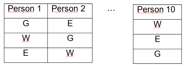
Important observations: It should be remembered that the block variable does not interact with the factors under study. It can be determined that the model is of absolute random blocks, when in each block all possible treatments are considered (it can also be a multiple of that number) and treatments are randomly assigned within each block. Many times all the treatments cannot be assigned in each block and that is when we find incomplete random block designs. It is assumed that the number of experimental units for each block must coincide with the number of treatments multiplied by the number of blocks, this implies that there is an observation corresponding to each level crossing between the block and the factor.
Completely random block design
This type of randomized complete block design is used when the researcher has the need to exercise local control with respect to variation and because there is a material that is experimentally heterogeneous, since otherwise (when it is homogeneous) uses completely randomized design (blocks are not required). The steps to be followed by the researcher for the completely randomized block design are:
- The researcher must use some criterion for grouping those homogeneous experimental units to generate the blocks, for example, they can be grouped by: methods, age, race, weight, sex, are the, litters, country, among others.
- Once the blocks have been formed, the treatments are randomly assigned to the experimental units in each block. In this way, a treatment is randomly assigned to each experimental unit.
- The blocks must be defined according to homogeneous experimental units, but which are within themselves, while they must be heterogeneous between one block and another.
- All treatments must be represented in the blocks and the idea is to minimize the variation within each block and maximize the inequalities between blocks.
Advantages of the randomized complete block experimental design
It increases the precision of the test since it eliminates one of the sources of variation of the error and that precision is measured by means of a coefficient of variation.
If the treatments are equal to the experimental units (or a multiple of them), this design allows great flexibility if there is no relationship between treatment and block.
In case of loss of information either by treatment or by block, in the same way the statistical analysis is not difficult.
The “principle of confusion” can be applied by matching the variables that have an influence on the response, but are ultimately not part of the interest of the researcher.
Disadvantages of the random full block design
It is not advisable for a large number of treatments, the recommendation ranges between 6 and 24 treatments.
It is also not recommended if there is a great variation in the experimental material, that is, when there is more than one variable.
When the effect of the block is not very significant, the degrees of freedom with respect to the error are unnecessarily decreased and it leads to a decrease in precision.
In the event that there is an interaction between treatment and block, the F test must be invalidated and this design cannot be applied.
Regarding the disturbing factor, we can say that the design most likely has an effect on the response that does not interest us and this disturbing factor can be in several ways:
Unknown disturbing factor and also not controllable, this factor can have different levels of variables while we carry out the experiment. The solution to this problem is randomization, since in this way the levels and possible effects of this factor are distributed in all the experimental units.
Disturbing factor that is known but not controllable, in this case a compensation can be made through the analysis of covariance, but only in the case that it can be observed in each run of the experiment, the value that this disturbing factor takes.
Known and controllable disturbing factor, in this case the solution may be the formation of blocks and in this way, statistical comparisons in the treatments are eliminated.
The completely randomized block design is one of the simplest to work in research and we will use it when we have at least 3 treatments, since if we only have two treatments, it is best to use a completely random design and the blocks do not they are necessary, since what is required is only a comparison between two groups.
We now go to the statistical model for the completely randomized block design, whose formula is the following:
Yij = µ + ti + ßj + Ԑij
The nomenclature to use is:
Yij = Observations obtained with the i-th treatment in the j-th repetition of the experiment.
µ = It is the general mean
ti = The effect of the i-th treatment
ßj = It is the effect of the j-th block
Ԑij = The experimental error of the i-th treatment in the j-th repetition
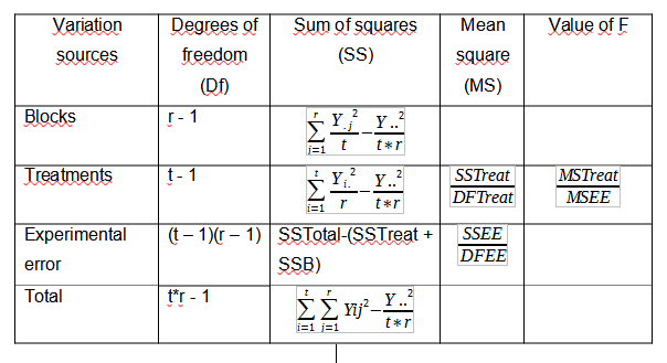
In a previous article we found the usefulness of analysis of variance (ANOVA). Where we can obtain results given by the sources of variation, the sums of squares, the degrees of freedom, the squares of the means of each component, as well as the value of F.
Variance analysis
Let’s go with an illustrative example: Let us suppose that we have a field and according to the characteristics of the place and the environment where the research is going to be carried out, it is that we are going to use a completely random design or a completely random block design.
Given the case that we are in an absolutely controlled, closed laboratory environment, such as a greenhouse and we have all the experimental units, we can use a completely randomized and balanced design (without blocks). But if we have lost some experimental units, we must work with a completely random but unbalanced design.
What happens if on my land I have a gradient, soil effect, terrain topography or simply certain conditions surrounding the investigation that can directly affect the final results, in this case we must use a completely block design at random, since it is specifically the blocks that will allow me to develop the research successfully, since they are capable of removing those disturbing factors that may be affecting the study.
Suppose we do a soil analysis and we realize that one part of the land of our research has less phosphorus, potassium, nitrogen and therefore is less fertile than the other and also, we are going to plant corn and we are going to apply a fertilizer in different doses, to see what is the amount of fertilizer that generates greater productivity.


But in this case, there is a serious disadvantage if we intend to use the completely random design when measuring the productivity of corn plants, since as each of the variables (treatments) is going to be placed at random, we can face a big problem. Because if precisely by chance of fate one of the treatments or doses of fertilizer is concentrated in the area of less fertility, our conclusions will be affected. We are now going to show a design where several treatments have been applied at random, to clarify the aforementioned.
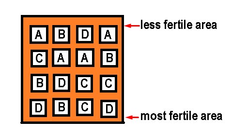
As we can see, we could come to the conclusion that treatment A does not generate higher productivity, but if we realize that treatment A is concentrated in the area with fewer nutrients and in reality its lack of productivity may not be due to the treatment in yes, but because of the soil where it was planted, so the results will be altered by that disturbing factor, which in this case is the level of soil fertility. For this reason, this type of design cannot be applied in this case, because it does not correct the factor of the difference in fertility in different areas of the same soil.
Of course, the ideal would be for all the land to have the same fertility conditions, but since this is not the case, we must use a completely random block design to try to block this disturbing factor, which does not allow us to know exactly which of the Fertilizer dose is the one with the highest productivity.
For this, the first thing we must do is have my general linear model of the completely random block design well defined and for this the following formula is used:
Yij = µ + ti + ßj + Ԑij
Where we know that Yij is the response variable that will be a function of the general mean (µ) + the effect of the treatments (ti) + the effect of the block (ßj) + the experimental error associated with each experimental unit.
Yij In this case, it will be the performance of the corn plant that will depend on each of these elements, being the sources of variation in my research those that are established in the previous formula.
The general mean (µ) that production capacity of the corn plant, regardless of the amount of fertilizer applied to it, is what the plant produces under natural conditions and without treatments.
The effect of the treatment (ti) will be the doses of fertilizer that are expected to be tested in the corn plant, to increase its yield and in this case, in each treatment it is established as:
A = 2gr
B = 4gr
C = 8gr
D = 10gr
Bj is the effect of the j-th block
Eij is the experimental error, since no matter how controlled the environmental conditions are at the laboratory level and foci with adequate light have been provided, humidity is intervened, etc. there will always be an experimental error. For example, if doses of hormones are applied, by human error a very small portion of difference can be introduced or perhaps a data taken in a wrong way and each of these factors are part of the experimental error.
The next step is to try to remove the disturbing effect and for this we will use a systematic randomization, the ideal would be that all the treatments are homogeneously concentrated in the whole field, that is, that one treatment is not more concentrated than another in the areas of higher or lower fertility. Ideally, the four treatments are evenly disaggregated in both areas, to be able to measure each of them under equal conditions and for this, it will be necessary to use a formula to find the number of repetitions. In the experimental design that we showed previously as an example of a completely random design (without blocks), we established 4 repetitions of each treatment, solely for a didactic purpose and because it is a simpler representation. But the number of repetitions (r) in the completely randomized block design must be calculated.
On the other hand, we already know that the number of treatments (t) is 4 and the formula for the degrees of freedom of the error (DFE) is given by:
DFE = (t - 1) (r - 1)
The degrees of freedom of the error will indicate the value in which I am going to dilute all the variations of my investigation and as a general rule the number 12 is established as a minimum. So that in this way the variation of the results can be divide effectively, so in general we will always work with this value when assuming the degrees of freedom of the error, although it is true that you can work with values greater than 12, here we are going to limit ourselves to this number.
Substituting the values in the formula, we can solve for the number of repetitions:
12 = (4 - 1) (r - 1)
12 = 3 (r - 1)
12 = 3rd - 3
r = 15/3 = 5
The experimental units, for this case, will be 5 repetitions multiplied by 4 treatments, that is, 20 experimental units.
Once we know the number of repetitions, we can plan the design of blocks completely at random, if there are 5 repetitions and they must be homogeneously distributed in each of the areas from lowest to highest fertility, we can establish a gradient in this sense and the Blocks must be oriented perpendicular to the direction of the gradient. So there should be one block for each repetition and 4 treatments in each block.
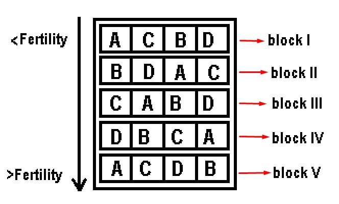
This time randomness will be in the arrangement of the treatments in each block, unlike the figure that represented the completely random design, where the treatments were randomly scattered throughout the field. With this block design, we correct the perturbation factor so that it does not affect the results of our experiment. This is because each level of the soil is fertile or not, there will be each of the treatments and then we can measure the effect of the treatments eliminating the disturbing factor, since there will be the same number of treatments for each level of the land and you will be able to measure how each of the treatments works in each of the different fertility zones.
We now go with a second example where we are going to use the ANOVA table to reach definitive conclusions.
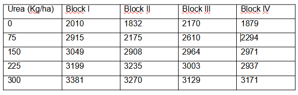
An experimental study was carried out to observe the dry matter yield in kg / ha with different contributions of N2 in the form of urea. The doses used were: 0 (as control doses), 75, 159, 126 and 300 Kg / ha and the study was carried out in different areas, in which different yields could be expected for climatic reasons. Importantly, the zones in this case acted as blocks.
The results obtained by treatment and by block are presented below:
The null hypothesis is stated as that there are no significant differences between the treatments, that is, that all the treatments are the same, while the alternative hypothesis, in contrast to the null hypothesis, is stated as that at least one of the treatments has significant differences with the rest or rather, not all treatments are the same.
Ho = t = ti
Ha = t ≠ ti
Applying the formula for the randomized complete block design we have:
Yij = µ + ti + ßj + Ԑij
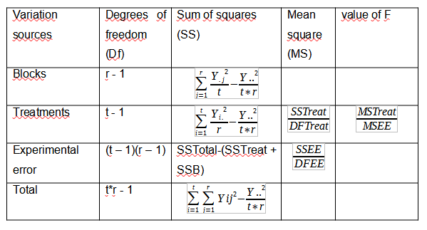
The ANOVA table will be as follows:
Variance analysis
Being “r” the number of repetitions, which in this case is equal to 4 (one for each block) and “t” the number of treatments that are 5.
We are going to find the elements that make up the sum of squares formula and show where they come from.
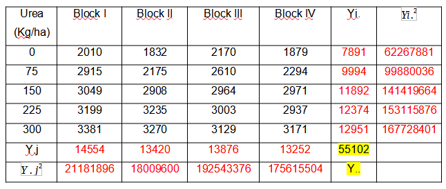
As we can observe:
Y.j = It is the sum of the treatments in each block
= Are the values of Y.j squared
Yi. = It is the sum of all the blocks for each treatment
= They are the values of Yi. squared
Y.. = It is the sum of all the treatments in each block with all the blocks in each treatment (it is underlined in yellow) and it is equivalent to the number of experimental units.
We are going to make the calculations of the sum of squares of both treatments and blocks, the experimental error and the totals, whose formulas come from the analysis of variance to be able to calculate the mean of the squares of the treatments and the experimental error. Once calculated, we can get to obtain F, which is a value that I can compare and will allow us to make a decision.
SSB =
= 203319
SSTreat =
= 4291444
SSTotal==
4804480
SSEE= SSTotal-(SSTreat + SSB) = 4804480 – 4291444 – 203319 = 309717
MSTreat =
= 1072861,08
MSEE =
= 25809,7
F = =
= 41,57
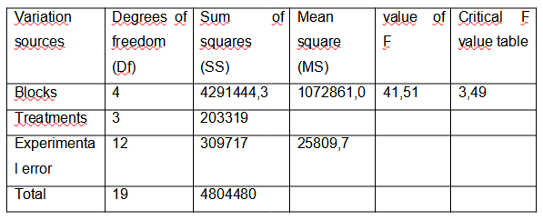
We are going to summarize the results of the analysis of variance in a table
We look for the critical value of F in tables where the numerator is the degree of freedom of the treatments = 3 and the denominator is the degree of freedom of the experimental error = 12
As we can see, according to the table the critical value of F = 3.49 with a significance level of 0.05 (which is the one usually used).
To make the decision, it is necessary to compare the obtained value of F with the critical value of F, if the value of F> critical value of F, the null hypothesis is rejected, in this case:
41.51> 3.49
This implies that the null hypothesis is rejected and therefore the alternative hypothesis is validated
Conclusions: According to the calculations, there is sufficient evidence that indicates a significant difference in terms of the yield of dry matter in at least one of the treatments, so it is recommended to evaluate which or which of the treatments are the ones that are presenting significant differences.
Other random block designs
Regarding the randomized block design, there are other types of designs, in addition to the completely randomized block design, where each treatment is applied in each block only once, it is important to mention that there is also the generalized randomized block design, where at As in the previous design, all treatments appear in each block, but in this design they can occur more than once.
It should be noted that there is also the incomplete block design, which is characterized in that not all treatments occur in each block and these in turn can be classified into:
- Balanced incomplete block design
- Partially balanced incomplete block design
- Incomplete block design with balanced treatment
- Latice design
- Extended block design: when each block has the same number of experimental units and is also greater than the number of treatments.
- Trend Free block design.
Generalized Randomized Block Design
This type of design is considered as an extension of the randomized complete block design and its difference with the previous one is that treatments are repeated in the same block, while in the previous design, the treatments occur only once per block.
It is also used when a disturbing factor is detected in the experimental units, but it is also applied when a treatment block interaction cannot be considered.
Advantages of this design
In addition to having all the advantages that the randomized complete block design has, it has the advantage that it is not required to have an independence between blocks and treatments.
Disadvantages
In the same way as the advantages, this design has the same disadvantages as the randomized complete block design, but also has an alternative restriction, which is that the number of repetitions within each block of the different treatments must be the same for all blocks, since otherwise, we could be within what is considered an unbalanced complete block design.
The model in this case is defined as:
Yijk = μ + ti + βj + TBij + Eijk
Where:
Yijk = this value corresponds to the i-th treatment of the j-th block that belongs to the k-th observation
μ = It is the general average that is common to all observations
ti = It is the effect produced by the i-th treatment
βj = Is the effect produced by the j-th block
TBij = The effect produced by the interaction of the block per treatment
Eijk = The experimental error